ELECTRONICS LAB

Sunday, December 22, 2013

Digital Locking System Using Microcontroller 89C52/89S52

If you are a beginner in making micro controller projects then this mini project
might just work for you. It's very simple and anybody can make it. The aim
of the project is quite predictable from the title itself-you enter a wrong password
the application wont work(in this case led is used as the application) and on correct
entering of the password, the application as in this case "led" will glow.In this Digital locking system project you will learn more about interfacing keypad and 16x2 LCD to your micro controller along with the code.

components required

For this project you will need the following components:

1 microcontroller 89C52(89S52 will also do)
1 potentiometer-10k
2 ceramic capacitors-22pF
1 switch(button for reset purpose)
1 electrolytic capacitor-10uF,25V
1 crystal oscillator-11.0592MHz
16x2 LCD display
1 resistor-10k
1keypad(here, i have used a calculator keypad.In proteus you can find it by typing keypad-smallcalc)
1 led
1 330 ohm resistor

Schematic diagram

Since this project has been made in proteus software you must have a prior knowledge of it. If you are unaware of the software here is a tutorial which i recommended in one of my previous articles.

The connection of the circuit is explained below:

Port 1 of the microcontroller is used as the output port
Port 2 of the microcontroller is used as the output port
Port 3 of the microcontroller is used as the input port.
The LCD is connected to port 2 since output is displayed on LCD
The led is connected to port 1 which is our application in this project
The keypad is connected to port 3
Other components like the crystal and switch are connected for the working of the microcontroller ( minimum circuitry required for proper working of the microcontroller).

working:

As soon as the power supply is provided to the microcontroller "password based" will be shown on the screen.This will remain for a second and after that "enter password" will be displayed as shown below.

The "ENTER PASSWORD " statement will remain for a second and then it will vanish.At this point you will have to enter password which will be shown in terms asterisk " **** ".

The coding of the micro-controller is done such that only four numbers can be used to enter password. If you want to increase the length of the password you can do that by adding loops in the coding which will be dealt later. Here, in this project the password is set as 1234. when this password is entered the LCD will display "correct password" as shown below and the LED will turn on which is connected at port 1. you can set your own password by changing the password in the code.

If you want to set your password using the operators like " + ", " -" etc you can do it by setting the password in the code as follows:

for " ON/C " =16
for " + " =10
for " - " =14
for " = " =15
for " x " =11
for " ÷ " =13

programming:

The programming of the microcontroller is done using keil compiler.The codings for this project is explained below:

#include "REGX51.H"

#include "delay.h" /*the header file of delay is added*/

#include "lcd.h" /*the header file of LCD is added*/

#include "keypad.h" /*the header file of keypad is added*/

#define relay P1_7;

void main()

{

int first_key,second_key,third_key,fourth_key;

P1=0X00; /*port 1 is defined as the output port*/

P2=0x00; /*port 2 is defined as the output port*/

P3=0xff; /*port 3 is defined as the input port*/

LCD_INIT();/* the LCD display is initialized */

LCD_STRING("PASSWORD BASED");/*displays PASSWORD BASED on the lcd*/

delay_sec(1); /* provides a delay of 1 second */

LCD_CMD(PUTLINE2);

LCD_STRING("LOCKING SYSTEM");

LCD_CLEAR(); /*clears the LCD display*/

LCD_STRING("ENTER PASSWORD:");

delay_sec(1);

LCD_CLEAR();

while(key_get()==NOKEY);

first_key=key;

LCD_STRING("*"); /*when any key is pressed display it as " * " */

while(key_get()==NOKEY);

second_key=key;

LCD_STRING("*");

while(key_get()==NOKEY);

third_key=key;

LCD_STRING("*");

while(key_get()==NOKEY);

fourth_key=key;

LCD_STRING("*"); /* by adding another while loop you can further increase the length of your password */

while(1)

{

if((first_key==1)&&(second_key==2)&&(third_key==3)&&(fourth_key==4))/*here, the password set is 1234. you can change the password over here.if you have increased your password length see that you also make changes in the If loop over here i.e by adding further &&fifth_key=....&& sixth_.. and so on */

{

LCD_CLEAR();

LCD_STRING("Correct Password");

P1_2=1; /* if correct password is entered make P1_2 high which will turn on the led */

delay_sec(2);

}

else

{

LCD_CLEAR();

LCD_STRING("Incorrect Password");

delay_sec(2);

}

} }

\\\\related topics\\\

Electronics Lab Created By Muhammad Irfan

Friday, December 13, 2013

Types of Relays

1 comment:

Types of Relays

In this article, the different types of relays like overload protection relay, solid state relay, solid state contactor relay, Buchholz relay, Mercury Wetted relay and many more are explained with diagrams. .

In my earlier post I have alreaady explained the working of relays, and their design and construction.

TAKE A LOOK : WORKING OF RELAYS

TAKE A LOOK : HOW TO TEST A RELAY

Now, let us take a look at the types of relays that are available for industrial use.

Basic Relays

Before going on to a deeper classification of the relays there are some basic relay circuits that must be kept in our mind. They are

Voltage Suppression Relays

As relays are used in industrial purposes very often, they are mostly controlled with the help of computers. But when relays are controlled with such devices, there will surely be the presence of semi-conductors like transistors. This will in turn cause the presence of voltage spikes. As a result, it is really necessary to introduce voltage suppression devices, otherwise they will clearly destroy the transistors.

This voltage suppression can be introduced in two ways. Either the computer provides the suppression or the relay provides the suppression. If the relay provides the suppression they are called voltage-suppression relays. In relays voltage suppression is provided with the help of resistors of high value and even diodes and capacitors. Out of these diodes and resistors are more commonly used. Whatever device is used, it will be clearly stated in the relay. Take a look at the diagram of a voltage suppressed relay with the help of a diode.

: voltage suppression relay using diode

De-spiking Diode Relays

A diode in the reverse-biased position is connected in parallel with the relay coil. As there is no flow of current due to such a connection, an open circuit of the relay will cause the current to stop flowing through the coil. This will have effect on the magnetic field. The magnetic field will be decreased instantly. This will cause the rise of an opposite voltage with very high reverse polarity to be induced. This is mainly caused because of the magnetic lines of force that cut the armature coil due to the open circuit. Thus the opposite voltage rises until the diode reaches 0.7 volts. As soon as this cut-off voltage is achieved, the diode becomes forward-biased. This causes a closed circuit in the relay, causing the entire voltage to pass through the load. The current thus produced will be flowing through the circuit for a very long time. As soon as the voltage is completely drained, this current flow will also stop. Take a look at the figure given below.

: De-spiking diode relays

De-spiking Resistor Relays

A resistor is almost efficient as that of a diode. It can not only suppress the voltage spikes efficiently, but also allows the entire current to flow through it when the relay is in the on position. Thus the current flow through it will also be very high. To reduce this, the value of the resistance should be as high as 1 Kilo Ohm. But, as the value of the resistors increases the voltage spiking capability of the relay decreases. Take a look at the circuit diagram below to understand more.

: De-spiking resistor relays

Types Of Relays

Here is a detailed list of the different types of relays.

1. Latching Relay

Latching relays are also called impulse relays. They work in the bistable mode, and thus have two relaxing states. They are also called keep relays or stay relays because as soon as the current towards this relay is switched off, the relay continues the process that it was doing in the last state. This can be achieved only with a solenoid which is operating in a ratchet and cam mechanism. It can also be done by an over-centre spring mechanism or a permanent magnet mechanism in which, when the coil is kept in the relaxed point, the over-centre spring holds the armature and the contacts in the right spot. This can also be done with the help of a remanent core.

In the ratchet and cam method, power consumption occurs only for a particular time. Hence it is more advantageous than the others.

2. Reed Relay

These types of relays have been given more importance in the contacts. In order to protect them from atmospheric protection they are safely kept inside a vacuum or inert gas. Though these types of relays have a very low switching current and voltage ratings, they are famous for their switching speeds.

3. Polarized Relay

This type of relay has been given more importance on its sensitivity. These relays have been used since the invention of telephones. They played very important roles in early telephone exchanges and also in detecting telegraphic distortion. The sensitivity of these relays are very easy to adjust as the armature of the relay is placed between the poles of a permanent magnet.

4. Buchholz Relay

This relay is actually used as a safety device. They are used for knowing the amount of gas present in large oil-filled transformers. They are designed in such a way that they produce a warning if it senses either the slow production of gas or fast production of gas in the transformer oil.

5. Overload protection Relay

As the name implies, these relays are used to prevent the electric motors from damage by over current and short circuits. For this the heating element is kept in series with the motor. Thus when over heat occurs the bi-metallic strip connected to the motor heats up and in turn releases a spring to operate the contacts of the relay.

6. Mercury Wetted Relay

This relay is almost similar to the reed relay explained earlier. The only difference is that instead of inert gases, the contacts are wetted with mercury. This makes them more position sensitive and also expensive. They have to be vertically mounted for any operation. They have very low contact resistance and so can be used for timing applications. Due to these factors, this relay is not used frequently.

7. Machine Tool Relay

This is one of the most famous industrial relay. They are mainly used for the controlling of all kinds of machines. They have a number of contacts with easily replaceable coils. This enabkes them to be easily converted from NO contact to NC contact. Many types of these relays can easily be setup in a control panel. Though they are very useful in industrial applications, the invention of PLC has made them farther away from industries.

8. Contacor Relay

This is one of the most heavy load relay ever used. They are mainly used in switching electric motors. They have a wide range of current ratings from a few amps to hundreds. The contacts of these relays are usually made with alloys containing a small percentage of silver. This is done so as to avoid the hazardous effects of arcing. These type of relays are mainly categorized in the rough use areas. So, they produce loud noises while operated and hence cannot be used in places where noise is a problem.

9. Solid State relay

SSR relays, as its name implies are designed with the help of solid state components. As they do not have any moving objects in their design they are known for their high reliability.

10. Solid State Contactor Relay

These relays combine both the features of solid state relays and contactor relays. As a result they have a number of advantages. They have a very good heat sink and can be designed for the correct on-off cycles. They are mainly controlled with the help of PLC, micro-processors or microcontrollers.

**Related Topics *

Electronics Lab Created By Muhammad Irfan

Introduction to MATLAB Tutorial

No comments:

In this article, we are giving an introduction to MATLAB. This article is part of a tutorial series we are developing for MATLAB. We hope you to give us feedback, so that we can improve our MATLAB tutorial series.

What does MATLAB stand for?

MATLAB stands for MATrix LABoratory. Hence, as the name suggests, here you play around with matrices. Using MATLAB an image (or any other data like sound, etc.) can be converted to a matrix and then various operations can be performed on it to get the desired results and values. Image processing is quite a vast field to deal with. We can identify colors, intensity, edges, texture or pattern in an image. In this tutorial, we would be restricting ourselves to detecting colours (using RGB values) only.

Getting acquainted with MATLAB environment

For those who have just finished installing MATLAB on their system and can’t figure out from where to start, no need to worry! This tutorial will first make you well acquainted with its very basics and then move further.

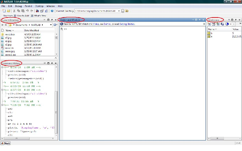
So, a typical MATLAB 2009 window looks like the image shown below.

MATLAB - 2009 - Home Screen

As marked in the image, there are 4 main windows.

Command window: This is the main window where you write the commands, as well as see the outputs. In other words, here is your interaction with the software.

Command History: As the name suggests, it shows the list of the commands recently used in chronological order. Hence, you can double click on a command to execute it again.

Current directory: It is the default directory (folder) for saving your files. All the files which you make (like m-files, as discussed later) are saved here and can be accessed from here directly. The location of the current directory is shown in the toolbar at the top. You can change it by changing the address here.

MATLAB - Change Directory Path

Workspace: It displays the list of the variables defined by you in the current session of MATLAB.

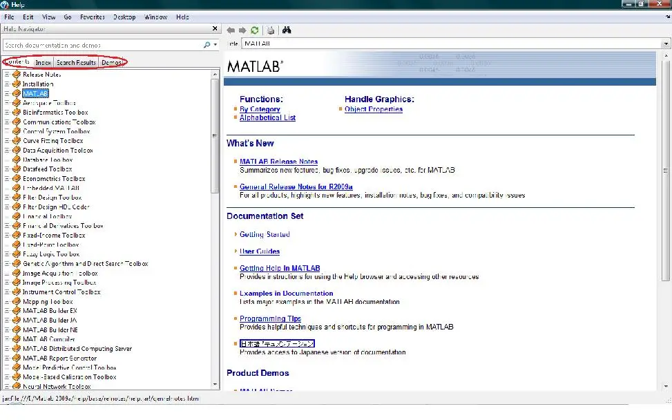
The Menu bar and Toolbar: The toolbar has buttons for common operations like cut, copy, paste, undo, redo. The most important button here is the HELP button. It opens the MATLAB help window which looks as the screenshot given below.

MATLAB - Help Page

You can get the details of any MATLAB command/function here and many demos of some commonly used applications. Locate the four tabs: Contents, Index, Search Results and Demos on the left. One of the best ways to learn by yourself is to look for demos of your interest and type the command/ function which you encounter there as the search term. You will then get the complete details of the function like its use, syntax, as well as few examples on how to use it. You can also have a look at some of the related functions at the end of page under the heading “See Also”. The demos related to Image Processing can be found under Image Processing Toolbox and Image Acquisition Toolbox.

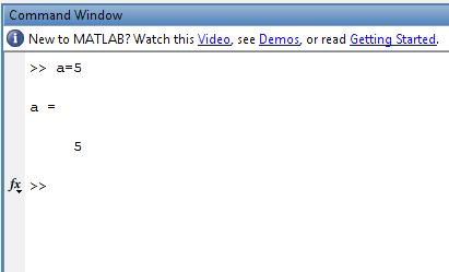
Now once we are done with knowing the essential features of MATLAB, let’s start typing something in the command window, say: a=5 and press enter.

Yes… as you can see that MATLAB creates a variable with name ‘a’, stores value 5 in it and displays it in the command window itself. Hence you can see how user-friendly MATLAB is.
Variables are stored in the form of Matrices in MATLAB. Hence, ‘a’ is a 1X1 matrix in the above example. Similarly, you can make one dimensional, two dimensional, etc. matrices as follows:

>> a=[1 3 5 7 9]
a =
1    3    5    7    9
>> b=[1 2 3;4 5 6;7 8 9]
b =
1    2    3
4    5    6
7    8    9

To avoid the display of the variable, we use semi-colon (;) at the end of instruction.

>> b=[1 2 3;4 5 6;7 8 9];

The indices of matrices in MATLAB start from 1 (unlike C/C++ and Java where they start from 0). We refer to a particular element of the matrix by giving its indices in parenthesis ().

>> b(2,1)
ans =4

Now with the variables in hand, you can perform various mathematical operations on them directly.

>> a=[1 2 3];
>> b=[6 7 8];
>> a+b
ans =
7 9 11

ans is the default variable of MATLAB. You can also store the result in another variable as

>> c=a+b c =
7 9 11

General functions & commands in MATLAB

clc: To clear the command window, giving you a ‘clear screen’.
clear: To remove all variables from the workspace. This frees up system memory.

Trigonometric functions

For angle in radians-

>> sin(1)
ans =0.8415

For angle in degrees

>> sind(30)
ans =0.5000

Inverse trigonometric-

>> asin(1)
ans =1.5708
>> asind(.5)
ans =30.0000

Similarly we have cos(), cosd(), acos(), tan() and other functions.

The Colon Operator

The colon is one of the most useful operators in MATLAB. It can create vectors, subscript arrays, and specify for iterations. In a very crude language, we can say that the colon (:) means “throughout the range”.

j:k                     is the same as [j,j+1,...,k]

j:i:k                   is the same as [j,j+i,j+2i, ...,k] A(:,j)                 is the jth column of A
A(:,j:k)              is A(:,j), A(:,j+1),…,A(:,k)

A(:)                   is all the elements of A, regarded as a single column.

Example:

>> a= [1 2 3; 4 5 6; 7 8 9]
a =
1    2    3
4    5    6
7    8    9

>> a(:,2:3)
ans =
2    3
5    6
8    9

Relational Operators

Operator	Description
==	Equal to
~=	Not equal to
<	Less than
<=	Less than or equal to
>	More than
>=	More than or equal to

Frequently used Functions & Commands

Conditional Statements

if, else: Execute statements if condition is true, false respectively.
Syntax:

if condition1 statement
elseif condition 2 statement
else
statement end

Example:

a=10;
>> if a<10 b=a/2;
else
b=a*2;
end
>> b
b =20

*Note: As a block is contained in braces {} in C/C++/Java, a block is terminated by the ‘end’statement in MATLAB.

LOOP-ing Commands

for: To create a loop – that is to execute a block of code specified number of times.
Syntax:

for variable = initval:endval statement
… statement
end

Example

>>c=[1 2 3 4 5]; b=0;
>>for i=1:5 b=b+c(i); end
>> b
b =15

while: Again to create loop, that executes till a specified condition is true.
Syntax:

while condition statements
end

Example:

>> c=2009; i=1; while c>1 b(i)=mod(c,10); c=c/10; i=i+1; end
>> b
b =9.0000 0.9000 0.0900 2.0090

zeros(): Create array/matrix of all zeros.
B = zeros(n) returns an n-by-n matrix of zeros.
B = zeros(m,n) returns an m-by-n matrix of zeros. Example,

>> z=zeros(2,4)
z =

0
0

0
0

0
0

0
0

Similarly we have ones() function for all values 1.
size(): Returns matrix dimensions.
Example:
for the above matrix z,

>> size(z)
ans =
2 4

length(): Returns the length of a vector. For an array, it returns the size of the longest dimension.
Example:

>>x = ones(1,8);
>>n = length(x)
n =8

dot(): Returns dot product of two vectors.
Example:

C = dot(A,B)

sqrt(): Returns square root of each element of an array
min(): Returns smallest elements in an array.
Syntax:

C = min(A)

If A is a matrix, min(A) treats the columns of A as vectors, returning a row vector containing the minimum element from each column. Similarly we have max() function.
sort(): Sorts array elements in ascending or descending order
Syntax:

B=sort(A,mode)

where value of mode can be

‘ascend’ : Ascending order (default)
‘descend’ : Descending order

plot(): Creates a 2-D line plot

So these all are the frequently used functions/commands in MATLAB. Until we come with our next chapter in MATLAB tutorial series, please share this article with your friends. Give us your feedback on improving the tutorial as well, we value it!

Image Representation in MATLAB – How to Represent Binary,Grayscale & Color Images

No comments:

Image Representation in MATLAB – How to Represent Binary,Grayscale & Color Images

In this article, we are going to talk about images, their types and some basic functions for Images. This article is part of our MATLAB tutorial series, which we are developing for Image processing through MATLAB. We expect you to give us feedback, so that we can keep the information flow more efficient, informative and up to the mark. In the first chapter, you have learned an introduction to MATLAB and its commands. In this chapter you will learn how to represent different types of images in MATLAB. In addition you will learn how to read & display images in MATLAB and how to create an M file.

Taking Up Images

Technically whatever we categorize as a picture, is an Image. We already talked about the basics of Image processing in our first article, we would focus today on technical representation of images.

Different Types of Images

Binary Image: An image that consists of only black and white pixels. Technically these types of images are called as Black and White Image. (Although it makes me sad to break my reader’s heart but till now what you called black and white images have some other technical name).

Grayscale Image: In daily language what we refer to as black-and-white (as in old photos) are actually grayscale. It contains intensity values ranging from a minimum (depicting absolute black) to a maximum (depicting absolute white) and in between varying shades of gray. Typically, this range is between 0 and 255.

Color Image: We all have seen this! Such an image is composed of the three primary colors, Red, Green and Blue, hence also called an RGB image.

Binary Image

Grayscale Image

Color Image

RGB value: All colors which we see around us can be made by adding red, blue and green components in varying proportions. Hence, any color of the world can uniquely be described by its RGB value, which stands for Red, Blue and Green values. This triplet has each value ranging from 0 to 255, with 0 obviously meaning no component of that particular color and 255 meaning full component. For example, pure red color has RGB value [255 0 0], pure white has [255 255 255], pure black has [0 0 0] and

has RGB value [55 162 170].

Representation of an Image in MATLAB

An image in MATLAB is stored as a 2D matrix (of size mxn) where each element of the matrix represents the intensity of light/color of that particular pixel. Hence, for a binary image, the value of each element of the matrix is either 0 or 1 and for a grayscale image each value lies between 0 and 255. A color image is stored as an mxnx3 matrix where each element is the RGB value of that particular pixel (hence it’s a 3D matrix). You can consider it as three 2D matrices for red, green and blue intensities.

Reading and Displaying Images

imread(): To read an image and store in a matrix.
Syntax: IM=imread(‘filename’)

where IM is a matrix. If the file is in the current directory (as described above), then you only need to write the filename, else you need to write the complete path. Filename should be with extension (.jpg, .bmp,..). There are some default images of MATLAB like ‘peppers.png’, ‘cameraman.tif’, etc. You can try reading them as

>>im=imread(‘peppers.png’);

It is always advised to use a semi-colon (;) at the end of the statement of reading an image, otherwise… you can try yourself what happens!

imshow(): Displays the image. Syntax:
imshow(‘filename’)
or imshow(im)

Example:-

>>imshow(‘cameraman.tif’);

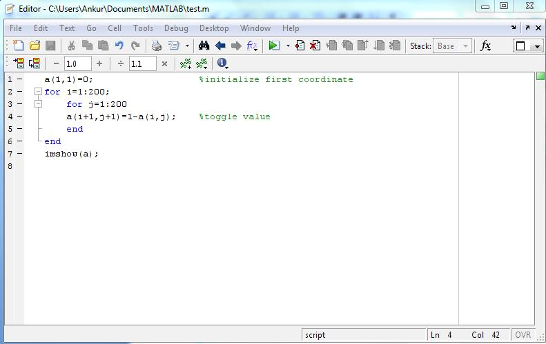
OK, now let’s make our own image, try this:

>>a(1,1)=0;
>>for i=1:200; for j=1:200
a(i+1,j+1)=1-a(i,j);
end end
>>imshow(a);

You try out making many different types of images like this just to make yourself comfortable with the commands learnt till now.

Data cursor: To see the values of the colors in the figure window, go to Tools>Data Cursor (or select from the toolbar), and click over any point in the image. You can see the RGB values of the pixel at location (X,Y).

A better option of data cursor is the function imtool(). Type the following

>>imtool(‘peppers.png’);

And see the pixel info on lower left corner as you move mouse pointer over different pixels.
Now, before we move on to our next article, we take a little detour in this article and talk about some MATLAB resources which will be extensively be used in coming article.

Making M Files & Functions in MATLAB

It is a provision in MATLAB where you can execute multiple commands using a single statement. Here the group of commands is stored as a MATLAB file (extension .m).

M Files in MATLAB - How to create & save an M File in Matlab

Here we have saved the m-file by the name “test.m”. Now as you type

>>test

And in MATLAB command window, all the above commands will execute.

Comments: As we have comments in C/C++/ Java using double slash (//), in MATLAB we use symbol % to write comments, i.e., statements that are not considered for execution. You can see comments in green in the snapshot above.

Functions in MATLAB

Functions, as some of you might know, are written to organize the code efficiently and make debugging easier. The set of statements within a function can be executed as and when required by just calling it, thereby avoiding repetitions. The data which is needed within the function can be passed as arguments and then the required values can be returned. You can return any no. of values and they can be matrices also.

We value your suggestions and feedback very much. Please drop by your comments. This encourages us to move forward!
Until next article is up this all folks! Keep reading and keep learning.

Electronics Lab Created By Muhammad Irfan

Types of Relays

No comments:

Types of Relays

In my earlier post I have alreaady explained the working of relays, and their design and construction.

TAKE A LOOK : WORKING OF RELAYS

TAKE A LOOK : HOW TO TEST A RELAY

Now, let us take a look at the types of relays that are available for industrial use.

Basic Relays

Before going on to a deeper classification of the relays there are some basic relay circuits that must be kept in our mind. They are

Voltage Suppression Relays

: voltage suppression relay using diode

De-spiking Diode Relays

: De-spiking diode relays

De-spiking Resistor Relays

: De-spiking resistor relays