Introduction to MATLAB Tutorial

In this article, we are giving an introduction to MATLAB. This article is part of a tutorial series we are developing for MATLAB. We hope you to give us feedback, so that we can improve our MATLAB tutorial series.

What does MATLAB stand for?

MATLAB stands for MATrix LABoratory. Hence, as the name suggests, here you play around with matrices.  Using MATLAB an image (or any other data like sound, etc.) can be converted to a matrix and then various operations can be performed on it to get the desired results and values. Image processing is quite a vast field to deal with. We can identify colors, intensity, edges, texture or pattern in an image. In this tutorial, we would be restricting ourselves to detecting colours (using RGB values) only.

Getting acquainted with MATLAB environment

For those who have just finished installing MATLAB on their system and can’t figure out from where to start, no need to worry! This tutorial will first make you well acquainted with its very basics and then move further.

So, a typical MATLAB 2009 window looks like the image shown below.

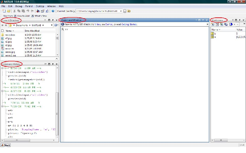
MATLAB - 2009 - Home Screen

As marked in the image, there are 4 main windows.

Command window: This is the main window where you write the commands, as well as see the outputs. In other words, here is your interaction with the software.

Command History: As the name suggests, it shows the list of the commands recently used in chronological order. Hence, you can double click on a command to execute it again.

Current directory: It is the default directory (folder) for saving your files. All the files which you make (like m-files, as discussed later) are saved here and can be accessed from here directly. The location of the current directory is shown in the toolbar at the top. You can change it by changing the address here.

MATLAB - Change Directory Path

Workspace: It displays the list of the variables defined by you in the current session of MATLAB.

 The Menu bar and Toolbar: The  toolbar  has  buttons  for  common  operations  like  cut,  copy,  paste,  undo,  redo.  The  most important button here is the HELP button. It opens the MATLAB help window which  looks as the screenshot given below.

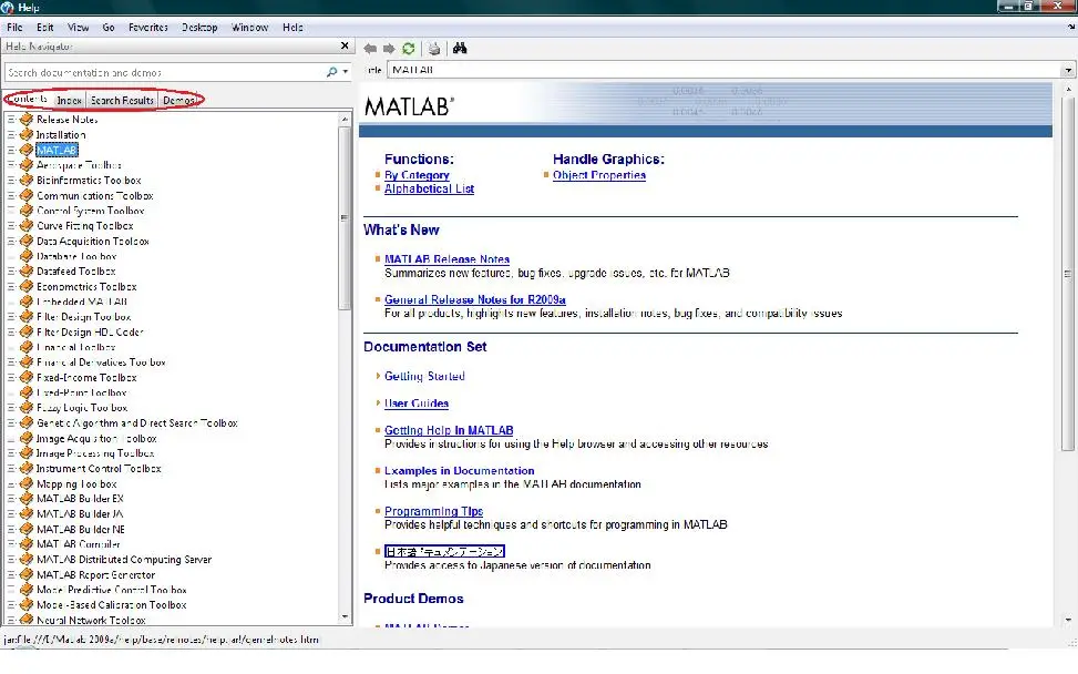
MATLAB - Help Page

 You can  get  the  details  of  any  MATLAB  command/function  here  and  many  demos  of  some commonly used applications. Locate the four tabs: Contents, Index, Search Results and Demos on the left. One of the best ways to learn by yourself is to look for demos of your interest and type the command/ function which you encounter there as the search term. You will then get the complete details of the function like its use, syntax, as well as few examples on how to use it. You can also have a look at some of the related functions at the end of page under the heading “See Also”. The demos related to Image Processing can be found under Image Processing Toolbox and Image Acquisition Toolbox.

Now once we are done with knowing the essential features of MATLAB, let’s start typing something in the command window, say: a=5 and press enter.

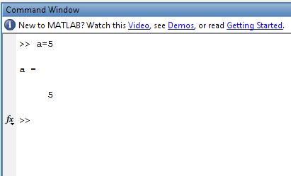
Yes… as you can see that MATLAB creates a variable with name ‘a’, stores value 5 in it and displays it in the command window itself. Hence you can see how user-friendly MATLAB is.
Variables are stored in the form of Matrices in MATLAB. Hence, ‘a’ is a 1X1 matrix in the above example. Similarly, you can make one dimensional, two dimensional, etc. matrices as follows:

>> a=[1 3 5 7 9]
a =
1     3     5     7     9
>> b=[1 2 3;4 5 6;7 8 9]
b =
1     2     3
4     5     6
7     8     9

To avoid the display of the variable, we use semi-colon (;) at the end of instruction.

 >> b=[1 2 3;4 5 6;7 8 9];

The indices of matrices in MATLAB start from 1 (unlike C/C++ and Java where they start from 0). We refer to a particular element of the matrix by giving its indices in parenthesis ().

>>  b(2,1)
ans =4

Now  with  the  variables  in  hand,  you  can  perform  various  mathematical  operations  on  them directly.

 >> a=[1 2 3];
>> b=[6 7 8];
>> a+b
ans =
7     9    11

ans is the default variable of MATLAB. You can also store the result in another variable as

 >> c=a+b c =
7     9    11

General functions & commands in MATLAB

clc: To clear the command window, giving you a ‘clear screen’.
clear: To remove all variables from the workspace. This frees up system memory.

Trigonometric functions

For angle in radians-

 >> sin(1)
ans =0.8415

For angle in degrees

>> sind(30)
ans =0.5000

Inverse trigonometric-

 >> asin(1)
ans =1.5708
>> asind(.5)
ans =30.0000

Similarly we have cos(), cosd(), acos(), tan() and other functions.

The Colon Operator

The colon is one of the most useful operators in MATLAB. It can create vectors, subscript arrays, and  specify  for  iterations.  In  a  very  crude  language,  we  can  say  that  the  colon  (:)  means “throughout the range”.

j:k                      is the same as [j,j+1,...,k]

j:i:k                    is the same as [j,j+i,j+2i, ...,k] A(:,j)                  is the jth column of A
A(:,j:k)               is A(:,j), A(:,j+1),…,A(:,k)

A(:)                    is all the elements of A, regarded as a single column.

Example: 

>> a= [1 2 3; 4 5 6; 7 8 9]
a =
1     2     3
4     5     6
7     8     9

>> a(:,2:3)
ans =
2     3
5     6
8     9

Relational Operators

Operator	Description
==	Equal to
~=	Not equal to
<	Less than
<=	Less than or equal to
>	More than
>=	More than or equal to

Frequently used Functions & Commands

Conditional Statements

if, else: Execute statements if condition is true, false respectively.
Syntax:

if condition1 statement
elseif condition 2 statement
else
statement end

 Example:

a=10;
>> if a<10 b=a/2;
else
b=a*2;
end
>> b
b =20

*Note:  As  a  block  is  contained  in braces  {}  in  C/C++/Java,  a block  is  terminated  by  the  ‘end’statement in MATLAB.

LOOP-ing Commands

for: To create a loop – that is to execute a block of code specified number of times.
Syntax:

for variable = initval:endval statement
… statement
end

Example 

>>c=[1 2 3 4 5]; b=0;
>>for i=1:5 b=b+c(i); end
>> b
b =15

while: Again to create loop, that executes till a specified condition is true.
Syntax:

while condition statements
end

 Example:

>> c=2009; i=1; while c>1 b(i)=mod(c,10); c=c/10; i=i+1; end
>> b
b =9.0000    0.9000    0.0900    2.0090

zeros(): Create array/matrix of all zeros.
B = zeros(n) returns an n-by-n matrix of zeros.
B = zeros(m,n) returns an m-by-n matrix of zeros. Example,

>> z=zeros(2,4)
z =

0	0	0	0
0	0	0	0

Similarly we have ones() function for all values 1.
size(): Returns matrix dimensions.
Example:
for the above matrix z,

>> size(z)
ans =
2     4

length(): Returns the length of a vector. For an array, it returns the size of the longest dimension.
Example:

>>x = ones(1,8);
>>n = length(x)
n =8

dot(): Returns dot product of two vectors.
Example:

C = dot(A,B)

sqrt(): Returns square root of each element of an array
min(): Returns smallest elements in an array.
Syntax:

C = min(A)

If A is a matrix, min(A) treats the columns of A as vectors, returning a row vector containing the minimum element from each column. Similarly we have max() function.
sort(): Sorts array elements in ascending or descending order
 Syntax:

B=sort(A,mode)

where value of mode can be

‘ascend’  :           Ascending order (default)
‘descend’ :           Descending order

plot(): Creates a 2-D line plot

So these all are the frequently used functions/commands in MATLAB. Until we come with our next chapter in MATLAB tutorial series, please share this article with your friends. Give us your feedback on improving the tutorial as well, we value it!

Image Representation in MATLAB – How to Represent Binary,Grayscale & Color Images

Image Representation in MATLAB – How to Represent Binary,Grayscale & Color Images

 

In this article, we are going to talk about images, their types and some basic functions for Images. This article is part of our MATLAB tutorial series, which we are developing for Image processing through MATLAB. We expect you to give us feedback, so that we can keep the information flow more efficient, informative and up to the mark. In the first chapter, you have learned an introduction to MATLAB and its commands. In this chapter you will learn how to represent different types of images in MATLAB. In addition you will learn how to read & display images in MATLAB and how to create an M file.

Taking Up Images

Technically whatever we categorize as a picture, is an Image. We already talked about the basics of Image processing in our first article, we would focus today on technical representation of images.

Different Types of Images 

Binary Image: An image that consists of only black and white pixels. Technically these types of images are called as Black and White Image. (Although it makes me sad to break my reader’s heart but till now what you called black and white images have some other technical name). 

Grayscale Image: In  daily  language  what  we  refer  to  as  black-and-white  (as  in  old  photos)  are  actually grayscale. It contains intensity values ranging from a minimum (depicting absolute black) to a maximum (depicting absolute white) and in between varying shades of gray. Typically, this range is between 0 and 255.

Color Image: We all have seen this! Such an image is composed of the three primary colors, Red, Green and Blue, hence also called an RGB image.

Binary Image

Grayscale Image

Color Image

RGB  value:  All  colors  which  we  see  around  us  can  be  made  by  adding  red,  blue  and  green components in varying proportions. Hence, any color of the world can uniquely be described by its RGB value, which stands for Red, Blue and Green values. This triplet has each value ranging from 0 to 255,  with  0  obviously  meaning  no component  of  that particular  color and  255  meaning  full component. For example, pure red color has RGB value [255 0 0], pure white has [255 255 255], pure black has [0 0 0] and   has RGB value [55 162 170].

Representation of an Image in MATLAB

An image in MATLAB is stored as a 2D matrix (of size mxn) where  each element  of the matrix represents the intensity of light/color of that particular pixel. Hence, for a binary image, the value of each element of the matrix is either 0 or 1 and for a grayscale image each value lies between 0 and 255. A color image is stored as an mxnx3 matrix where each element is the RGB value of that particular pixel (hence it’s a 3D matrix). You can consider it as three 2D matrices for red, green and blue intensities.

Reading and Displaying Images

imread(): To read an image and store in a matrix.
Syntax: IM=imread(‘filename’)

where IM is a matrix. If the file is in the current directory (as described above), then you only need to write the filename, else you need to write the complete path. Filename should be with extension (.jpg, .bmp,..). There are some default images of MATLAB like ‘peppers.png’, ‘cameraman.tif’, etc. You can try reading them as

>>im=imread(‘peppers.png’);

It is always  advised  to use a semi-colon  (;)  at  the end  of the  statement  of reading  an  image, otherwise… you can try yourself what happens!

imshow(): Displays the image. Syntax:
imshow(‘filename’)
or imshow(im)

Example:-

>>imshow(‘cameraman.tif’);

OK, now let’s make our own image, try this:

>>a(1,1)=0;
>>for i=1:200; for j=1:200
a(i+1,j+1)=1-a(i,j);
end end
>>imshow(a);

You try out making many different types of images like this just to make yourself comfortable with the commands learnt till now.

Data cursor: To see the values of the colors in the figure window, go to Tools>Data Cursor (or select from the toolbar), and click over any point in the image. You can see the RGB values of the pixel at location (X,Y).

A better option of data cursor is the function imtool(). Type the following

 >>imtool(‘peppers.png’);

And see the pixel info on lower left corner as you move mouse pointer over different pixels.
Now, before we move on to our next article, we take a little detour in this article and talk about some MATLAB resources which will be extensively be used in coming article.

Making M Files & Functions in MATLAB

It is a provision in MATLAB where you can execute multiple commands using a single statement. Here the group of commands is stored as a MATLAB file (extension .m).

Here we have saved the m-file by the name “test.m”. Now as you type

>>test

And in MATLAB command window, all the above commands will execute.

Comments: As we have comments in C/C++/ Java using double slash (//), in MATLAB we use symbol %  to  write  comments,  i.e.,  statements  that  are  not  considered  for  execution.  You can see comments in green in the snapshot above.

 Functions in MATLAB

Functions,  as  some  of  you might  know,  are  written  to organize  the  code  efficiently  and  make debugging easier. The set of statements within a function can be executed as and when required by just calling it, thereby avoiding repetitions. The data which is needed within the function can be passed as arguments and then the required values can be returned.  You can return any no. of values and they can be matrices also.

 We value your suggestions and feedback very much. Please drop by your comments. This encourages us to move forward!
Until next article is up this all folks! Keep reading and keep learning.


























 Electronics Lab  Created By Muhammad Irfan